|
|
||||||
|
|
Home| Journals | Statistics Online Expert | About Us | Contact Us | |||||
 |
||||||
| About this Journal | Table of Contents | ||||||
|
|
[Abstract] [PDF] [HTML] [Linked References] Control of Chaos in Some Non Linear Maps Tarini Kumar Dutta1*, Debasish Bhattacharjee2† 1Gauhati University, Guwahati, Assam 781014 INDIA 2B.Borooah College, Guwahati, Assam 781007 INDIA Corresponding Addresses: *[email protected], †[email protected] Research Article Abstract: In this paper we have considered two non linear ecological maps which are chaotic in nature beyond accumulation points. First of all Chau’s method is applied on both of these maps and the chaotic region is controlled forming periodic trajectories. The set of initial points are obtained which help in converging to the periodic points. Again the periodic pulse method discussed by Matias and Guemez has been applied on the same and the chaotic nature is controlled. Key Words: Chaos, Periodic orbits, Accumulation point 2010 AMS Classification: 37 G 15, 37 G 35 ,37 C 45
Chaos occurs in many models representing real world system, for example chemical system may exhibit chaotic behavior if they contain certain elements of dynamical feedback. Chaos had been shown to exist in fluid dynamics such as Raleigh Bernard convection, in non linear optics, in electronics such as Chua’s circuit e.t.c. Chaos is observed as undesirable part in engineering control practice. So, controlling of chaos is an essential part of study of chaos. Since 1990 chaos control problem attracts researchers and engineers. The first control technique was OGY method[17] proposed by Ott et.al in 1990.After that several hundreds of techniques have been added in these decades. We have taken the periodic proportional pulse method[2,13] to control chaos in generalized logistic map. The proportional pulse method was discussed by Matias and Guemez[13] . After that N.P.Chau[2] discussed in a similar manner but gave some restrictions on the initial conditions by which chaos can be controlled . However he has also shown that for large periodic value sometimes chaos is suppressed and sometimes not . In section 1.2 we have applied Chau’s method on one dimensional generalized logistic map. The considered map[4,8] is xn+1=a xnk(b-c xnr) for b=c=1, r=0.1, K=0.5 , where “a” is the variable parameter. It has been observed that chaotic region starts for a >14.3700933623526….. We consider the parameter value a = a0(say)=14.9 which is beyond the accumulation point and shows a chaotic attractor. In section 1.3 the same technique is applied on two dimensional ecological model[3,11,15,16] at the parameter value beyond the accumulation point,. In section 1.4 proportional pulse method as discussed by Matias and Guemez is applied on the above said one dimensional and two dimensional maps for controlling chaos.
1.2 One dimensional map and controlling of chaos: Theory of Chau’s technique is as follows. Let x* be one of the periodic points of period p. Then x*=fp(x*). For stability we have For p=1 at a= a0 , the curve C1(x) is as follows:
Fig 1.2.a: The curve C1(x), y=1 and y= -1.The figure shows positive values of x for which C1(x) lies between -1 and 1.
We take a value of x such that |C1(x)|<1(the above figure will help in choosing the value of x) and get the value of k satisfying equation (1.2.1). After solving the equation C1(x)= -1 by secant method, we have x=0.52446.Thus if the value of x which is to be made as the fixed point for the function F lies in the interval (0,0.52446), so that the fixed point becomes stable .We take x=0.5, using (1.2.1), the value of k=0.70866 for which x becomes a stable fixed point of F. Now if the value of k is applied at every iteration in the logistic like map the trajectory goes to the stable fixed point x.
Fig 1.2.b: Abscissa represents the number of iterations, while the ordinate represents the value of x at every iteration. In the figure 1.2.b, up to 20000 iterations it has been observed that chaos occurs, and after that the control is switched on, which shows that it converges to a point. The above calculation is done for p=1at a0. Similarly for p=2, C2(x) =
Fig 1.2.c: The curve C2(x), y=1 and y= -1.The figure shows positive values of x for which C2(x) lies between -1 and 1. After solving the equation C2(x) = -1, we have x=0.037412.Thus the range of possible stable fixed points for F is (0, 0.037412). We have taken a value of x such that |C2(x) |<1, and get the value of k satisfying equation (1.2.1) for p=2 . For x= 0.03 , k=0.0864857. Now we apply the value of k after every iteration in the logistic like map. The diagram is as follows:
Fig 1.2.d: Abscissa represents the number of iterations, while the ordinate represents the value of x at every iteration. Iteration is done up to 90000. After 60000 iterations the function F is injected after every iteration of f . Now, after 60000 iterations the next point if lies in the basin of attraction of the stable fixed point of F, the trajectory will converge to the stable fixed point of F. If x* is a fixed point of F, then k f2(x*)=x*. Let f(x*)=y*, therefore f(y*)=x*/k. The figure shows that the chaos is suppressed to form the periodic points of period two after 60000 iterations. Thus the stable periodic points when controlling parameter is switched on are {x*,y*}. Similarly at the parameter a=14.9, C4(x) is plotted.
Fig 1.2.e: The curve C4(x), y=1 and y= -1.The figure shows part of positive values of x for which C4(x) lies between -1 and 1. One of the possible ranges of stable fixed points is (0.000451243, 0.0157235) which is obtained on solving the equations C4(x) = -1 and C4(x) = 1. The value of x is taken as 0.015 and k=0.029969 is obtained using (1.2.1). So, if we take the value of x=0.015 which will be stable since min{(C4)-1(-1), (C4)-1(1)} The diagram showing control of chaos is as follows:
Fig 1.2.f: Abscissa represents the number of iterations, while the ordinate represents the value of x at every iteration. From the diagram it is clear that up to 60000 iteration that the trajectory does not follow any stable periodic orbit but after 60000 iteration periodic orbit of period 4 is followed, actually this is the region where chaos control period four is switched on. 1.3 One dimensional map and controlling of chaos: Now the extended version of the above process [3] is applied in the two dimensional ecological map f(x, y)=(
G=KFp, where K is a diagonal matrix whose diagonal elements are k1 and k2 and Fp represents composition of F, p times. Any fixed point of G let’s say X is stable if G=KFp (X)=X and Jacobian matrix has two eigen values whose modulus is less than unity. Now, we have to obtain the values of k1 and k2 such that chaos is controlled. We take the value of a=;b=0.01;k=;r=2.9; From chapter 3 it is clear that r=2.9 lies in the chaotic region. We consider p=1. Now the Jacobian matrix of (7.3.1) is as follows:
So, Jacobian matrix of G will be
i.e. So, characteristic polynomial is given by,
X= Some of the diagonal element= Y=determinant= The fixed points will be stable if where i.e. k1 = we pick those values of x, y which satisfies (1.3.2)
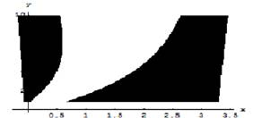
Fig1.3.a: The points(x, y) which satisfy both (1.3.2) and (1.3.3).
Fig1.3.b: Chaos is controlled by taking x=3.3,y= 4.91 from the shaded portion of fig 1.3.a. In fact up to 7000 iteration is done at the control parameter a=2.9 which shows the attractor is chaotic and after that controlling parameters are switched on. For other values of p , we have
Where xp-1=first component of fp-1 and yp-1 is the second component of fp-1 . And the Jacobian matrix is given as Some examples using different values of p following above discussed procedure are as follows: For p=2:
Fig 1.3.c: Abscissa is the x co-ordinate while ordinate is y co-ordinate of the point (x,y). Shaded portion represents (x, y) which may be a stable fixed point by taking suitable values k1,k2
Fig1.3.d: Abscissa is the number of iterations while ordinate is y co-ordinate of the point (x, y). Up to 3000 iteration is done at the control parameter a=2.9 which shows the attractor is chaotic and after that controlling parapmeters are switched on.
For p=4:
Fig 1.3.e: Abscissa is the x co-ordinate while ordinate is y co-ordinate of the point (x,y). Shaded portion represents (x, y) which may be a stable fixed point by taking suitable values k1,k2
Fig 1.3.f: Abscissa is the number of iterations while ordinate is y co-ordinate of the point (x, y). Up to 3000 iteration is done at the control parameter a=2.9 which shows the attractor is chaotic and after that controlling parameters are switched on.
For p=8:
Fig 1.3.g: Abscissa is the x co-ordinate while ordinate is y co-ordinate of the point (x,y). Shaded portion represents (x, y) which may be a stable fixed point by taking suitable values k1, k2 However it is difficult to control chaos even the points are taken from the shaded portions considering them as the stable fixed points as the basin of attraction of the fixed points considered are small . So, after some iterations if the controlling switch is switched on the initial point may not lie in the basin of attraction of the considered fixed points . 1.4 Controlling of chaos with Matias’ method: Another version of the above method is now applied. This process is to inject pulse let’s say For example after every fourth iteration a pulse is injected of the form xi+1=k xi , k=0.0001with an initial value 0.1 for the control parameter a=14.9 and the result is as follows:
Fig 1.4.a: Abcissa represents the number of iterations n while ordinate represents the value of x.
In the above figure up to 20000 iterations the trajectory shows chaotic behavior after which the controlling is switched on and it shows stable periodic points of period 4. However for the same values of the parameters if we take k=0.001 the result is as follows:
Fig 1.4.b: Abscissa represents the number of iterations n while ordinate represents the value of x. In the figure7.4.b up to 20000 iterations the trajectory goes free after which impulse is given at every fourth iteration. Again if the impulse is given after every three iterations with k=0.01keeping the other conditions same then the result is as follows:
Fig 1.4.c: Abscissa represents the number of iterations n while ordinate represents the value of x.
The above figure shows a stable periodic points of period three. Now we are giving the pulse after every two iterations for k=0.01 and the result is as follows:
Fig 1.4.d: Abscissa represents the number of iterations n while ordinate represents the value of x. Some of the observations bellow for different values of k keeping the other conditions same: For k = 0.09:
Fig 1.4.e: Abscissa represents the number of iterations n while ordinate represents the value of x. In the above figure iteration is done at the parameter 14.9. Up to 20,000 iterations it may be observed that chaos has occurred, after that periodic pulse is injected resulting control of chaos. For k=0.08:
Fig 1.4.f: Abscissa represents the number of iterations n while ordinate represents the value of x. From the above diagrams it has been observed that the periodic orbit is dependent on the iteration number on which the proportional pulse is injected(specially values of n=1,2,3). We extend the above idea and use it in two dimensional map: The considered two dimensional map is
It has been observed in chapter 3 that the chaotic region starts at r=2.7065672384929 when a=0.5105854,b=0.01,K=4.7913155.We take the parameter value of r= 2.9 which is ahead of the accumulation point. We inject pulse at every second iteration of the form The result is on n vs y[i]
Fig 1.4.g: Abscissa represents the number of iterations n while ordinate represents the value of y of the co-ordinate (x, y).
The result is shown on n vs x[i]
Fig 1.4.h: Abscissa represents the number of iterations n while ordinate represents the value of x of the co-ordinate (x, y). 1.5 Conclusion: The proposed method are applicable and effective to control chaos up to low periodic points. However it is difficult to maintain periodic points of period greater than eight as the basin of attraction of these periodic points become small and hence when the chaos control parameter is switched on the initial value may not fall in the basin of attraction of the stable periodic points. References:
|
|||||
|
||||||